How to Build a High-Performance Time-Series Database on OpenMetal

Time-series data is the lifeblood of modern digital operations. From IoT sensor networks generating millions of readings per second to financial systems tracking market movements in microseconds, organizations increasingly depend on the ability to capture, store, and analyze data points as they occur over time. Whether you’re monitoring application performance, tracking user behavior, analyzing financial markets, or managing industrial IoT deployments, the infrastructure hosting your time-series database directly impacts your ability to extract value from this data.

Building a high-performance time-series database requires more than selecting the right software, it demands infrastructure that can sustain the intense write throughput, deliver consistent query latency, and scale economically as your data volumes grow. This guide walks you through the fundamentals of time-series databases, explores popular open source options, and provides a practical blueprint for deploying a production-grade time-series architecture on OpenMetal’s bare metal infrastructure.

What Is a Time-Series Database?

A time-series database (TSDB) is a database system specifically designed to store, manage, and analyze data points that are indexed by time. Unlike traditional relational databases that excel at transactional workloads, time-series databases handle the unique characteristics of temporal data: high-volume writes, time-based queries, and the need for efficient storage compression.

Time-series data consists of measurements or observations captured at specific moments, whether at fixed intervals (such as sensor readings every 10 seconds) or irregular intervals (like server error logs that only record when events occur). Each data point typically includes a timestamp, one or more measured values, and metadata describing the source or context of the measurement.

Common examples of time-series data include:

• IoT sensor telemetry: Temperature, humidity, pressure, and vibration readings from industrial equipment or environmental monitors
• Financial market data: Stock prices, trading volumes, order book updates, and cryptocurrency exchange rates
• Application performance metrics: CPU usage, memory consumption, request rates, error counts, and response times
• User behavior analytics: Page views, click events, feature interactions, and conversion funnel progression
• Infrastructure monitoring: Network throughput, disk I/O, database query latencies, and container resource utilization

The defining characteristic of time-series data is that it changes continuously over time, enabling you to analyze trends, detect anomalies, and make predictions based on historical patterns.

Why Traditional Databases Struggle With Time-Series Workloads

Traditional relational databases like PostgreSQL and MySQL were designed for transactional workloads where data is frequently updated and queried in complex ways across multiple tables. This architecture works well when you need strong consistency guarantees and support for arbitrary queries, but it creates performance bottlenecks for time-series workloads.

Time-series databases are optimized to address several key challenges that traditional databases struggle with:

High write throughput: Time-series applications generate data continuously, often at rates of thousands or millions of data points per second. Traditional databases that maintain complex indexes and enforce ACID guarantees can’t sustain this level of write activity without significant hardware investment.

Storage efficiency: Time-series data exhibits patterns of similarity. Consecutive temperature readings differ by fractions of a degree, timestamps increment predictably, and metadata rarely changes. Specialized time-series databases apply compression techniques like delta encoding and columnar storage to reduce storage requirements by 10x or more compared to row-based relational databases.

Time-based query performance: Most time-series queries involve filtering by time ranges, grouping data into intervals (hourly averages, daily totals), and performing aggregations across time windows. Time-series databases optimize for these access patterns through time-based indexing and pre-aggregation strategies, while general-purpose databases must scan large portions of tables to answer the same queries.

Data lifecycle management: Time-series data has a natural lifecycle. Recent data requires millisecond query latency for real-time dashboards, while older data is accessed less frequently and can be downsampled or archived. Traditional databases lack built-in mechanisms for automatically managing this data temperature transition.

These architectural differences make time-series databases essential for workloads where data volume, write performance, and query efficiency are primary concerns.

Popular Open Source Time-Series Database Options

The open source ecosystem offers several mature time-series database solutions, each with distinct architectures and optimization trade-offs. Understanding the characteristics of these platforms helps you select the right tool for your specific use case.

InfluxDB

InfluxDB was one of the first mainstream time-series databases, launched in 2013 with a focus on developer experience and ease of deployment. It uses a custom query language (InfluxQL in version 1.x, Flux in version 2.x, and SQL in version 3.x) and provides features like continuous queries for automatic data downsampling and retention policies for automatic data expiration.

InfluxDB works well for single-server deployments and offers managed cloud options, but some users report stability challenges during version upgrades and when scaling to extremely high cardinality workloads.

Prometheus

Prometheus emerged from SoundCloud in the mid-2010s as an open source monitoring and alerting system designed specifically for cloud-native environments. It uses a pull-based model where Prometheus servers scrape metrics from instrumented applications, and it stores data locally on disk using a custom time-series database format.

Prometheus excels at monitoring use cases with its powerful PromQL query language, built-in alerting capabilities, and extensive integration ecosystem. However, Prometheus was designed as a monitoring solution rather than a long-term data warehouse. It doesn’t support clustering for horizontal scalability, and long-term data retention typically requires external storage systems.

TimescaleDB

TimescaleDB takes a different approach by building time-series optimizations as an extension to PostgreSQL rather than creating a new database from scratch. It automatically partitions data into time-based chunks called hypertables, applies columnar compression for storage efficiency, and adds time-series-specific SQL functions.

This approach provides full SQL compatibility, allows you to join time-series data with relational data in the same database, and benefits from PostgreSQL’s mature ecosystem. The trade-off is that you inherit PostgreSQL’s resource requirements and may not achieve the same write throughput as purpose-built systems for extremely high-velocity workloads.

ClickHouse

ClickHouse is a columnar OLAP database originally developed by Yandex for analytics workloads but widely adopted for time-series use cases. It uses a columnar storage format that enables high compression ratios and fast analytical queries across billions of rows.

ClickHouse supports standard SQL with extensive date/time functions, provides excellent performance for both writes and queries, and scales horizontally through its native clustering capabilities. Its versatility makes it suitable not just for time-series metrics but also for logs, traces, and event data, though it requires more operational expertise than simpler solutions.

Gnocchi

Gnocchi is an open source time-series database that takes a unique approach by aggregating data at ingestion time rather than at query time. This design decision means that Gnocchi pre-computes averages, minimums, maximums, and other aggregations as data arrives, making queries extremely fast since they only need to read back pre-computed results.

Gnocchi was specifically designed for cloud platforms and supports multi-tenancy, horizontal scalability, and pluggable storage backends. It’s particularly well-suited for OpenStack environments where it can integrate with the Ceilometer metering service for comprehensive infrastructure monitoring.

Key Requirements for Time-Series Database Infrastructure

Selecting the appropriate infrastructure for your time-series database has as much impact on performance as choosing the database software itself. Time-series workloads place specific demands on the underlying hardware and network that, when not properly addressed, create bottlenecks that no amount of software optimization can overcome.

Consistent I/O Performance

Time-series databases ingest data continuously, writing millions of small records to disk throughout the day. This access pattern differs fundamentally from batch processing workloads that write large files periodically. You need storage that can sustain high IOPS (input/output operations per second) without performance degradation, especially during peak ingestion periods.

Virtualized cloud storage often introduces performance variability due to resource contention with other tenants. One moment you’re achieving excellent write throughput, and the next your writes are being throttled because a neighbor is running an I/O-intensive workload. This unpredictability makes it difficult to size your infrastructure appropriately and can cause ingestion backlogs during critical periods.

Predictable Resource Allocation

Time-series queries range from simple point lookups (what was the temperature at 3:15 PM yesterday?) to complex aggregations spanning months of data (show me the 95th percentile response time for each service, grouped by hour, for the past quarter). These queries can consume significant CPU and memory resources, and you need confidence that those resources will be available when your analysts run their queries.

In shared virtualized environments, your database may be competing with other workloads for CPU cycles and memory bandwidth. This “noisy neighbor” problem means query performance becomes unpredictable. The same query might take 2 seconds during off-peak hours and 20 seconds during peak times, not because your data changed but because you’re resource-starved.

High-Bandwidth, Low-Latency Networking

Modern time-series architectures distribute data across multiple nodes for both high availability and horizontal scalability. ClickHouse replicates data between replicas for fault tolerance, TimescaleDB synchronizes hypertables across nodes, and Prometheus remote storage implementations stream metrics to long-term storage backends.

This inter-node communication happens continuously, not just during initial setup but throughout normal operations. A distributed ClickHouse cluster might be replicating gigabytes of data per hour between replicas while simultaneously serving queries that need to pull results from multiple shards. Network bandwidth and latency directly impact both data durability and query performance.

Flexible Storage Tiering

Time-series data has a natural temperature gradient. Recent data (the last few hours or days) gets queried frequently for real-time dashboards and requires sub-millisecond access latency. Older data (weeks or months old) is accessed less frequently, typically for trend analysis or compliance reporting, and can tolerate higher latency in exchange for lower storage costs.

You need infrastructure that supports multiple storage tiers with different performance and cost characteristics, along with the ability to implement data lifecycle policies that automatically move data between tiers as it ages. This could mean starting with NVMe SSDs for hot data, moving to traditional HDDs for warm data, and ultimately archiving to object storage for long-term retention.

Why OpenMetal’s Infrastructure Excels for Time-Series Databases

OpenMetal’s bare metal infrastructure addresses each of these requirements with an architecture specifically designed for high-performance data workloads, making it an ideal foundation for production time-series deployments.

Dedicated Resources Without Virtualization Overhead

Each OpenMetal bare metal server provides dedicated CPU cores, memory, and NVMe storage without the “noisy neighbor” interference common in virtualized public cloud environments. When you provision a server for your ClickHouse deployment, those resources are exclusively yours. No sharing, no contention, no performance surprises.

This resource isolation translates directly to predictable time-series database performance. Your ClickHouse, TimescaleDB, or InfluxDB workloads achieve consistent query response times and sustained write throughput even during peak ingestion periods. For applications processing millions of data points per second—whether IoT sensor networks, financial tick data, or application performance monitoring—this consistency is critical for maintaining service level agreements.

High-Bandwidth Unmetered Private Networking

OpenMetal servers include dual 10 Gbps network interfaces (20 Gbps aggregate bandwidth) with completely unmetered private east-west traffic between servers in your environment. This networking capacity enables high-performance distributed time-series architectures where clusters can:

• Replicate data between nodes for high availability without bandwidth charges impacting architectural decisions
• Distribute queries across shards for parallel processing, allowing you to scale query performance horizontally
• Synchronize state between coordinator and worker nodes in distributed query engines
• Stream data from ingestion pipelines to storage clusters without worrying about bandwidth costs

This unmetered private networking is particularly valuable for time-series workloads that generate continuous data streams. Whether you’re replicating ClickHouse data between replicas, streaming metrics from Prometheus remote storage, or syncing TimescaleDB hypertables across nodes, you can design your architecture for performance and reliability rather than optimizing to minimize network transfer costs.

Multi-Tiered Storage Strategy

OpenMetal’s infrastructure supports a comprehensive storage strategy that optimizes both performance and cost for time-series data lifecycle management:

High-performance NVMe drives provide the sub-millisecond query latency required for hot data, things like recent metrics powering real-time dashboards, operational monitoring views, and alerting rules. NVMe SSDs deliver the sustained IOPS necessary for time-series databases to maintain high write throughput while simultaneously serving read queries.

Cost-effective HDD arrays handle warm and cold data retention for historical analysis, trend identification, and compliance archives. While HDDs can’t match NVMe performance, they offer significantly lower cost per terabyte, making them ideal for data that’s queried less frequently but must remain accessible.

Ceph-based block and object storage provides S3-compatible endpoints for long-term time-series archival with built-in redundancy and custom erasure coding profiles. You can configure retention policies in your time-series database to automatically export older data to object storage, maintaining queryability while dramatically reducing storage costs.

OpenStack-Powered Flexibility

The OpenStack-powered platform supports both containerized Kubernetes deployments for orchestrated time-series services and direct bare metal installations. This flexibility lets you choose the deployment model that best fits your operational preferences—use Kubernetes for managing application-level services or deploy directly to bare metal for maximum performance.

Full root access to your bare metal servers enables time-series-specific optimizations that managed cloud platforms prohibit:

• Custom kernel tuning for network stack parameters that improve TCP performance for high-frequency time-series ingestion
• Filesystem selection and configuration based on your workload characteristics—XFS for high-concurrency writes, ext4 for compatibility, or ZFS for advanced features
• Direct NVMe configuration to minimize write amplification and extend SSD lifespan under heavy time-series workloads
• Memory allocation tuning for time-series compression algorithms that trade CPU for storage efficiency

High-memory configurations up to 2TB DDR5 RAM support in-memory caching of frequently queried time ranges, dramatically reducing disk I/O for dashboard queries and analytical workloads that repeatedly access recent data.

Predictable, Cost-Effective Pricing

OpenMetal’s fixed-cost pricing model eliminates the unpredictable expenses that plague time-series workloads on public cloud platforms:

• No per-IOPS charges for heavy write workloads that continuously ingest sensor telemetry or application metrics
• No premium storage tier costs for guaranteed performance—you get consistent NVMe performance at a fixed monthly rate
• No egress fees when querying data from visualization tools, streaming metrics to analytics platforms, or replicating between regions
• No API request charges for high-frequency ingestion patterns common in time-series applications

Customers building time-series databases for IoT sensor telemetry, financial market analytics, observability platforms, and application performance monitoring report 40-60% cost savings versus public cloud while achieving better P99 query latencies. The predictable monthly cost makes capacity planning straightforward and eliminates bill shock from unexpected usage spikes.

Time-Series-Specific Infrastructure Optimizations

OpenMetal’s infrastructure supports architectural patterns specifically beneficial for time-series databases:

Dedicated storage clusters with tunable replication factors let you balance data durability against storage efficiency. For metrics where some data loss is acceptable, you might use a replication factor of 2 to reduce storage costs. For financial data where every data point matters, you can configure replication factor 3 or implement erasure coding for maximum durability.

Network configurations supporting tens of thousands of concurrent connections accommodate the massively parallel ingestion workloads typical of time-series systems. IoT platforms might maintain persistent connections from millions of devices, each sending periodic readings, requiring infrastructure that can handle connection state at scale.

Colocation of time-series databases with analytical processing engines on the same private network enables zero-cost data movement during complex queries. You can run Apache Spark, Presto, or Apache Flink in the same environment as your ClickHouse cluster, allowing these engines to process time-series data directly without paying network egress fees or dealing with cross-region latency.

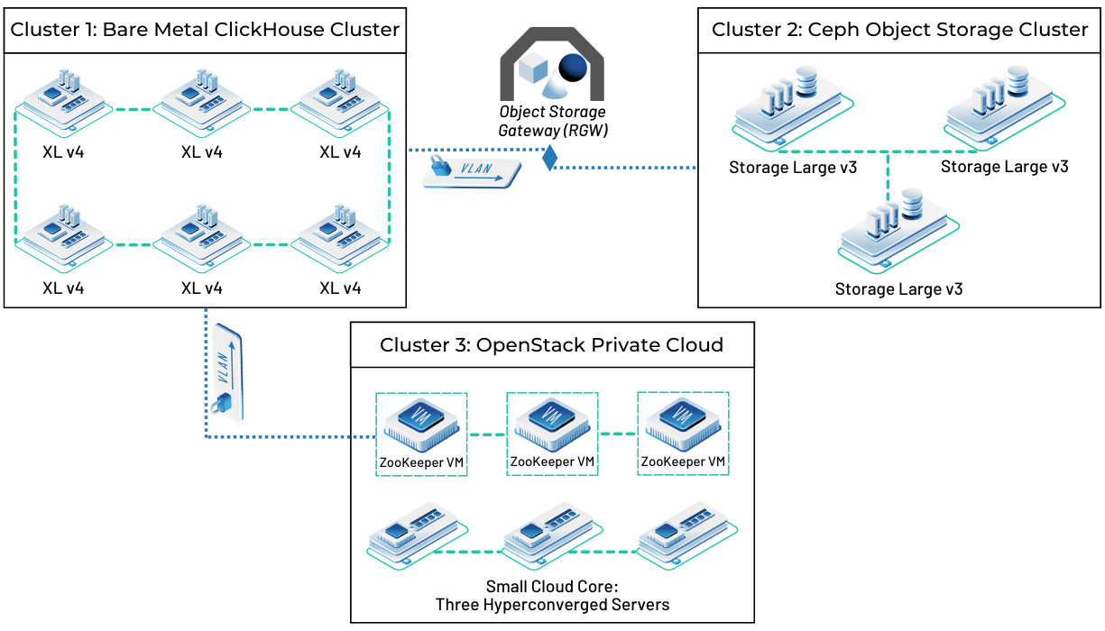
Architecture Blueprint: Building a ClickHouse Time-Series Database on OpenMetal

This section provides a detailed blueprint for deploying a production-grade ClickHouse time-series database on OpenMetal infrastructure. While the specific commands and configurations apply to ClickHouse, many of the architectural principles and infrastructure patterns are relevant regardless of which time-series database you choose.

Why ClickHouse for Time-Series Workloads

ClickHouse’s columnar storage architecture makes it particularly well-suited for time-series analytics. By storing each column separately and compressing similar values together, ClickHouse achieves 10-100x compression ratios on typical time-series data. This compression reduces not just storage costs but also I/O requirements, allowing queries to process billions of rows by reading only the relevant columns from disk.

ClickHouse’s query performance stems from several architectural decisions: vectorized query execution that processes data in batches rather than row-by-row, parallel processing that automatically distributes work across CPU cores, and specialized algorithms for different data types and query patterns. These optimizations enable ClickHouse to scan and aggregate billions of time-series data points in seconds on commodity hardware.

For distributed deployments, ClickHouse provides native clustering capabilities with automatic data distribution across shards and replication for high availability. The system handles query routing and result aggregation automatically, letting you scale horizontally by adding nodes to your cluster as your data volume grows.

Infrastructure Requirements and Server Specifications

For a production ClickHouse deployment handling millions of time-series data points per second, provision OpenMetal bare metal servers with the following specifications:

Cluster nodes (minimum 3 servers for high availability):

• CPU: 16-32 cores
• RAM: 128-256 GB DDR5
• Storage: 2-4 TB NVMe SSD for hot data, plus additional capacity for cold data
• Network: Dual 10 Gbps NICs

ZooKeeper coordination cluster (3 servers for quorum):

• CPU: 4-8 cores
• RAM: 16-32 GB
• Storage: 500 GB SSD
• Network: 10 Gbps NICs

The ClickHouse cluster nodes handle both data storage and query processing, while the ZooKeeper cluster coordinates distributed operations like replica synchronization and leader election. Separating ZooKeeper onto dedicated servers improves reliability and prevents resource contention.

Step 1: Prepare Your OpenMetal Environment

Begin by provisioning your bare metal servers through the OpenMetal cloud control panel. Select server configurations that match your anticipated data volume and query workload. For this guide, we’ll provision three ClickHouse nodes and three ZooKeeper nodes.

After provisioning completes, configure private networking between your servers. OpenMetal’s software-defined networking allows you to create isolated VLANs for inter-cluster communication, keeping your time-series data traffic separate from other workloads and external networks.

Configure your firewall rules to allow the following traffic between cluster nodes:

• ClickHouse native protocol (port 9000) for inter-node communication
• ClickHouse HTTP interface (port 8123) for client connections and monitoring
• ZooKeeper client port (2181) for coordination
• ZooKeeper peer communication ports (2888, 3888)

Step 2: Install and Configure ZooKeeper

ZooKeeper provides distributed coordination services that ClickHouse uses to maintain cluster metadata and coordinate replica operations. Install ZooKeeper on your three dedicated coordination nodes.

On each ZooKeeper server, install the ZooKeeper package:

sudo apt-get update
sudo apt-get install -y zookeeperd

Create a unique server ID for each ZooKeeper node by writing a number (1, 2, or 3) to the myid file:

echo "1" | sudo tee /var/lib/zookeeper/myid

Edit the ZooKeeper configuration file /etc/zookeeper/conf/zoo.cfg to define your cluster members:

tickTime=2000
dataDir=/var/lib/zookeeper
clientPort=2181
initLimit=10
syncLimit=5
server.1=zk1.yourdomain.local:2888:3888
server.2=zk2.yourdomain.local:2888:3888
server.3=zk3.yourdomain.local:2888:3888

Replace the hostnames with your actual ZooKeeper server addresses. Restart ZooKeeper on each node:

sudo systemctl restart zookeeper
sudo systemctl enable zookeeper

Verify that your ZooKeeper cluster formed successfully by checking the status:

echo stat | nc localhost 2181

You should see output indicating the node’s mode (leader or follower) and connection statistics.

Step 3: Install ClickHouse on Cluster Nodes

Install ClickHouse on each of your cluster nodes. For detailed installation instructions specific to OpenMetal, refer to our guide on how to install ClickHouse on OpenMetal Cloud.

On each ClickHouse node, add the ClickHouse repository and install the server package:

sudo apt-get install -y apt-transport-https ca-certificates dirmngr
sudo apt-key adv --keyserver hkp://keyserver.ubuntu.com:80 --recv 8919F6BD2B48D754

echo "deb https://packages.clickhouse.com/deb stable main" | sudo tee /etc/apt/sources.list.d/clickhouse.list
sudo apt-get update

sudo apt-get install -y clickhouse-server clickhouse-client

During installation, you’ll be prompted to set a password for the default user. Choose a secure password and record it for later use.

Step 4: Configure ClickHouse for Distributed Operations

ClickHouse’s configuration lives in XML files under /etc/clickhouse-server/. Create a remote servers configuration file that defines your cluster topology.

Create /etc/clickhouse-server/config.d/remote_servers.xml:

<yandex>
    <remote_servers>
        <timeseries_cluster>
            <shard>
                <replica>
                    <host>clickhouse1.yourdomain.local</host>
                    <port>9000</port>
                </replica>
                <replica>
                    <host>clickhouse2.yourdomain.local</host>
                    <port>9000</port>
                </replica>
            </shard>
            <shard>
                <replica>
                    <host>clickhouse3.yourdomain.local</host>
                    <port>9000</port>
                </replica>
            </shard>
        </timeseries_cluster>
    </remote_servers>

    <zookeeper>
        <node>
            <host>zk1.yourdomain.local</host>
            <port>2181</port>
        </node>
        <node>
            <host>zk2.yourdomain.local</host>
            <port>2181</port>
        </node>
        <node>
            <host>zk3.yourdomain.local</host>
            <port>2181</port>
        </node>
    </zookeeper>

    <macros>
        <shard>01</shard>
        <replica>replica1</replica>
    </macros>
</yandex>

This configuration creates a cluster with two shards, where the first shard has two replicas for high availability. Adjust the shard and replica values in the macros section for each server—each node should have a unique shard/replica combination.

Configure network access by creating /etc/clickhouse-server/config.d/network.xml:

<yandex>
    <listen_host>0.0.0.0</listen_host>
    <interserver_http_host>clickhouse1.yourdomain.local</interserver_http_host>
</yandex>

Set the interserver_http_host to the hostname of each specific node.

Restart ClickHouse on all nodes to apply the configuration:

sudo systemctl restart clickhouse-server
sudo systemctl enable clickhouse-server

Step 5: Create Time-Series Database Schema

Connect to any ClickHouse node using the client:

clickhouse-client --password

Create a database for your time-series data:

CREATE DATABASE IF NOT EXISTS timeseries ON CLUSTER timeseries_cluster;

Define a table using the ReplicatedMergeTree engine for data replication and the Distributed table engine for query routing. First, create the local replicated table on each shard:

CREATE TABLE timeseries.metrics_local ON CLUSTER timeseries_cluster
(
    timestamp DateTime,
    device_id String,
    metric_name String,
    metric_value Float64,
    tags Map(String, String)
)
ENGINE = ReplicatedMergeTree('/clickhouse/tables/{shard}/metrics', '{replica}')
PARTITION BY toYYYYMM(timestamp)
ORDER BY (device_id, metric_name, timestamp)
TTL timestamp + INTERVAL 90 DAY;

This table definition includes several important elements:

• Partitioning by month (PARTITION BY toYYYYMM(timestamp)) enables efficient data management and allows you to drop entire partitions when data expires
• Ordering by device_id, metric_name, and timestamp optimizes query performance for common access patterns
• TTL policy automatically deletes data older than 90 days, implementing your data retention requirements
• ReplicatedMergeTree engine ensures data is replicated across cluster nodes for high availability

Now create a distributed table that provides a single interface for inserting and querying data across all shards:

CREATE TABLE timeseries.metrics ON CLUSTER timeseries_cluster
AS timeseries.metrics_local
ENGINE = Distributed(timeseries_cluster, timeseries, metrics_local, rand());

When you insert data into the distributed table, ClickHouse automatically routes it to the appropriate shard based on the sharding key (in this case, a random distribution). When you query the distributed table, ClickHouse executes the query on all shards in parallel and aggregates the results.

Step 6: Optimize Storage Configuration

ClickHouse’s storage efficiency comes from its compression algorithms and encoding strategies. Configure additional storage optimizations for your time-series workload.

For columns with low cardinality (limited distinct values), use dictionary encoding:

ALTER TABLE timeseries.metrics_local 
MODIFY COLUMN device_id String CODEC(LZ4);

For numeric columns with predictable patterns, use delta encoding:

ALTER TABLE timeseries.metrics_local 
MODIFY COLUMN timestamp DateTime CODEC(Delta, LZ4);

These codecs reduce storage requirements without impacting query performance—in fact, queries often run faster because less data needs to be read from disk.

Step 7: Implement Data Tiering for Hot and Cold Storage

Time-series data naturally divides into hot data (recent, frequently accessed) and cold data (older, infrequently accessed). Implement a tiering strategy that stores hot data on fast NVMe drives and automatically migrates cold data to less expensive HDDs.

First, configure storage policies in /etc/clickhouse-server/config.d/storage.xml:

<yandex>
    <storage_configuration>
        <disks>
            <hot>
                <path>/var/lib/clickhouse/hot/</path>
            </hot>
            <cold>
                <path>/mnt/hdd/clickhouse/cold/</path>
            </cold>
        </disks>
        <policies>
            <tiered>
                <volumes>
                    <hot>
                        <disk>hot</disk>
                    </hot>
                    <cold>
                        <disk>cold</disk>
                    </cold>
                </volumes>
                <move_factor>0.2</move_factor>
            </volumes>
        </policies>
    </storage_configuration>
</yandex>

Update your table definition to use the tiered storage policy:

ALTER TABLE timeseries.metrics_local 
MODIFY SETTING storage_policy = 'tiered';

ClickHouse will now automatically move data partitions from hot to cold storage based on the move factor (when a volume reaches 80% capacity) and the time-based TTL settings.

Step 8: Configure Data Ingestion

Your time-series database is now ready to receive data. ClickHouse supports multiple ingestion methods depending on your data source and volume requirements.

For application metrics, you can use ClickHouse’s native protocol through client libraries available in most programming languages. Here’s an example Python script for inserting time-series data:

from clickhouse_driver import Client
import time

client = Client(host='clickhouse1.yourdomain.local', password='your_password')

metrics = [
    {
        'timestamp': int(time.time()),
        'device_id': 'sensor_001',
        'metric_name': 'temperature',
        'metric_value': 23.5,
        'tags': {'location': 'warehouse_a', 'zone': '1'}
    }
]

client.execute(
    'INSERT INTO timeseries.metrics (timestamp, device_id, metric_name, metric_value, tags) VALUES',
    metrics
)

For high-volume ingestion, batch your inserts to reduce overhead. Accumulate data points in memory and flush them in batches of 10,000-100,000 rows depending on your latency requirements.

For integrating with existing monitoring systems, ClickHouse supports Prometheus remote write protocol, allowing you to configure Prometheus to stream metrics directly to ClickHouse for long-term storage. Configure this in your Prometheus configuration:

remote_write:
  - url: "http://clickhouse1.yourdomain.local:8123/api/v1/write"
    basic_auth:
      username: default
      password: your_password

Step 9: Build Time-Series Queries and Dashboards

With data flowing into your ClickHouse cluster, you can now build queries to analyze your time-series data. ClickHouse’s SQL interface makes it straightforward to perform common time-series operations.

Calculate the average metric value grouped by hour:

SELECT 
    toStartOfHour(timestamp) AS hour,
    device_id,
    metric_name,
    avg(metric_value) AS avg_value
FROM timeseries.metrics
WHERE timestamp >= now() - INTERVAL 24 HOUR
GROUP BY hour, device_id, metric_name
ORDER BY hour DESC;

Identify the 95th percentile response time across all devices:

SELECT 
    toStartOfMinute(timestamp) AS minute,
    quantile(0.95)(metric_value) AS p95_latency
FROM timeseries.metrics
WHERE metric_name = 'response_time'
  AND timestamp >= now() - INTERVAL 1 HOUR
GROUP BY minute
ORDER BY minute DESC;

For visualization, ClickHouse integrates with popular tools like Grafana. Install the ClickHouse data source plugin in Grafana and configure a connection to your cluster. You can then build dashboards that query your time-series data in real-time, displaying metrics, alerts, and trends.

Step 10: Monitor Your ClickHouse Cluster

Monitor your ClickHouse deployment to ensure it maintains optimal performance as your data volume grows. ClickHouse exposes system tables that provide visibility into query performance, storage utilization, and replication status.

Check query performance by examining slow queries:

SELECT 
    query,
    query_duration_ms,
    read_rows,
    read_bytes
FROM system.query_log
WHERE type = 'QueryFinish'
ORDER BY query_duration_ms DESC
LIMIT 10;

Monitor replication lag to ensure replicas stay synchronized:

SELECT 
    database,
    table,
    replica_name,
    absolute_delay
FROM system.replicas
WHERE absolute_delay > 60;

Track storage utilization across your cluster:

SELECT 
    database,
    table,
    formatReadableSize(sum(bytes_on_disk)) AS size,
    sum(rows) AS rows
FROM system.parts
WHERE active
GROUP BY database, table
ORDER BY sum(bytes_on_disk) DESC;

Set up alerting rules in your monitoring system to notify you when replication lag exceeds acceptable thresholds, storage utilization reaches capacity limits, or query performance degrades.

Alternative Time-Series Database Architectures on OpenMetal

While this guide focused on ClickHouse, OpenMetal’s infrastructure supports a variety of time-series database architectures depending on your specific requirements and existing technology stack.

TimescaleDB for PostgreSQL Compatibility

If your organization has extensive PostgreSQL expertise or requires the ability to join time-series data with relational data in the same database, TimescaleDB offers an compelling alternative. Deploy PostgreSQL with the TimescaleDB extension on OpenMetal bare metal servers to achieve better performance than managed PostgreSQL services while maintaining full SQL compatibility.

The deployment process mirrors standard PostgreSQL installation with the addition of the TimescaleDB extension. You can then create hypertables that automatically partition your time-series data by time, implement compression policies to reduce storage costs, and use continuous aggregates to pre-compute common queries for dashboard performance.

InfluxDB for Developer-Friendly Time-Series Storage

For teams prioritizing simplicity and fast time-to-value, InfluxDB provides an easy-to-deploy time-series database with a straightforward data model and query language. Deploy InfluxDB on OpenMetal servers to avoid the high costs of InfluxDB Cloud while maintaining control over your data and infrastructure.

InfluxDB’s automatic data retention policies, built-in visualization capabilities through its admin UI, and extensive client library ecosystem make it accessible for teams without deep database administration expertise. The recent addition of SQL support in InfluxDB 3.0 further reduces the learning curve for SQL-familiar developers.

Prometheus for Monitoring-Focused Deployments

If your primary use case is infrastructure and application monitoring rather than long-term analytics, consider deploying Prometheus on OpenMetal infrastructure. While Prometheus wasn’t designed for long-term data retention, you can configure it with remote write to send data to ClickHouse, TimescaleDB, or object storage for historical analysis while maintaining Prometheus’ excellent alerting and real-time monitoring capabilities.

This hybrid approach combines Prometheus’ monitoring strengths with a separate time-series database for retention and analytics, giving you the best of both worlds without sacrificing either real-time alerting or long-term trend analysis.

Optimizing Time-Series Database Performance

Beyond selecting appropriate infrastructure and software, several operational practices significantly impact time-series database performance and cost efficiency.

Implement Appropriate Data Retention Policies

Not all time-series data requires permanent retention. Implement tiered retention policies that automatically downsample or delete data based on age and access patterns. Keep recent data at full granularity for detailed analysis while aggregating older data into hourly or daily rollups that preserve trends without storing every data point.

This approach reduces storage costs and improves query performance by limiting the volume of data that must be scanned for historical queries. A dashboard showing the last 24 hours of metrics at one-second granularity might query millions of data points, while the same dashboard showing last year’s trend using daily averages queries just 365 aggregated values.

Optimize Query Patterns for Time-Series Access

Time-series databases perform best when queries align with the data’s natural structure. Filter by time ranges first to limit the data processed, use indexes effectively by including indexed columns in WHERE clauses, and avoid queries that require sorting or grouping by non-time dimensions without also filtering by time.

Leverage materialized views or continuous aggregates to pre-compute common queries. If your dashboard displays the same hourly averages every time it loads, don’t recalculate those averages on every page view, create a materialized view that updates incrementally as new data arrives.

Monitor and Tune Compression Settings

Time-series data compresses remarkably well due to its temporal patterns and repetitive structure, but compression effectiveness varies based on encoding choices. Monitor your compression ratios and experiment with different codecs to find the optimal balance between compression efficiency and query performance.

Some codecs trade CPU time for better compression. This might be acceptable for cold data that’s rarely queried but counterproductive for hot data where query speed matters more than storage efficiency. Profile your queries to identify when decompression becomes a bottleneck and adjust codecs accordingly.

Plan for Growth and Scalability

Time-series data volumes grow linearly with time, making capacity planning more predictable than transactional workloads. Use your ingestion rate and planned retention period to project storage requirements, then provision infrastructure with headroom for growth.

OpenMetal’s infrastructure makes horizontal scaling straightforward: add new nodes to your cluster to increase storage capacity and query throughput. Because you’re not paying per-resource pricing, you can provision capacity proactively rather than reactively, avoiding performance degradation as you approach limits.

Real-World Time-Series Database Use Cases on OpenMetal

OpenMetal customers deploy time-series databases across diverse industries and use cases, each benefiting from the infrastructure’s performance characteristics and cost predictability.

IoT Sensor Networks and Industrial Monitoring

Manufacturing and industrial IoT deployments generate continuous streams of sensor data from equipment monitoring vibration, temperature, pressure, and performance metrics. These workloads require infrastructure that can sustain high write throughput as thousands or millions of sensors report readings simultaneously, often at sub-second intervals.

OpenMetal’s dedicated bare metal servers eliminate concerns about resource contention during data ingestion spikes, ensuring sensor data is captured reliably even during production peaks. The unmetered networking allows real-time data replication to multiple data centers for disaster recovery without incurring bandwidth charges that would make such architectures cost-prohibitive on public cloud platforms.

Financial Market Data and Trading Analytics

Financial services firms process massive volumes of market data—stock prices, order book updates, trade executions—that must be stored for regulatory compliance, backtesting trading strategies, and real-time market analysis. These workloads demand sub-millisecond query latency for real-time trading decisions combined with the ability to store years of historical data for trend analysis.

The consistent I/O performance and high-memory configurations available on OpenMetal bare metal servers enable in-memory caching of frequently accessed data while maintaining fast access to historical data on NVMe storage. Organizations report significantly better P99 query latencies compared to virtualized cloud platforms where storage performance varies unpredictably.

Application Performance Monitoring and Observability

Modern distributed applications generate telemetry data from every service, container, and function execution: metrics, logs, and traces that together provide visibility into application health and user experience. This observability data grows proportionally with application scale, and many organizations struggle with the escalating costs of storing this data on consumption-based cloud platforms.

By deploying observability infrastructure on OpenMetal, organizations eliminate per-IOPS charges for continuous metric ingestion, egress fees for dashboard queries, and premium storage tier costs for guaranteed performance. The fixed-cost model makes it economically feasible to retain observability data for extended periods, enabling deeper historical analysis and more accurate capacity planning.

User Analytics and Product Intelligence

Product teams instrument applications to track user behavior, feature usage, and conversion funnels all generating time-series data that informs product decisions. This data requires efficient storage for potentially hundreds of millions of users generating events continuously, combined with fast query performance for interactive dashboards and ad-hoc analysis.

The flexibility of OpenMetal’s infrastructure allows product analytics teams to deploy specialized time-series databases optimized for their query patterns while integrating them with data lakes and data warehouses for comprehensive analytics. The ability to collocate these systems on the same private network eliminates data movement costs and reduces latency for complex analytical queries.

Getting Started With Your Time-Series Database on OpenMetal

Building a production-grade time-series database requires thoughtful infrastructure choices that balance performance, scalability, and cost. OpenMetal’s bare metal infrastructure provides the foundation for time-series workloads that need consistent I/O performance, predictable resource allocation, high-bandwidth networking, and flexible storage tiering all at a fixed monthly cost that makes capacity planning straightforward.

Whether you choose ClickHouse for its analytical capabilities, TimescaleDB for PostgreSQL compatibility, InfluxDB for developer experience, or another time-series database, OpenMetal’s infrastructure delivers the performance characteristics these workloads demand without the unpredictable costs and resource contention of virtualized platforms.

The architecture patterns and optimization techniques in this guide apply across time-series database technologies, giving you a framework for building scalable, cost-effective time-series infrastructure regardless of which specific database you select. Start with understanding your data infrastructure options, evaluate your requirements for write throughput and query latency, and design your architecture to leverage OpenMetal’s strengths in dedicated resources, unmetered networking, and flexible storage.

For organizations processing millions of data points per second, storing terabytes or petabytes of historical data, and requiring sub-second query response times, the infrastructure hosting your time-series database matters as much as the database software itself. OpenMetal provides that infrastructure with predictable performance and transparent pricing that scales with your data growth.